Understanding the Roofline Model without the Roof (First)

A blog post explaining the Roofline model by starting from basic processor–memory interaction to motivate the X-axis (arithmetic intensity) and Y-axis (performance), then showing how optimizations move a kernel right or up on the plot, and finally introducing the memory-bandwidth and compute roofs that bound achievable performance.

Preface

A typical computing system consists of two main components: memory and a processor, as illustrated below. During program execution, data is fetched from memory into the processor, where computations are performed.

The rate at which data can be transferred between memory and the processor over the bus is measured in bytes per second (Byte/s). This is a property of the memory subsystem.

The rate at which the processor can execute operations is measured in operations per second (op/s). This is a property of the processor (CPU or GPU).

A typical computing system

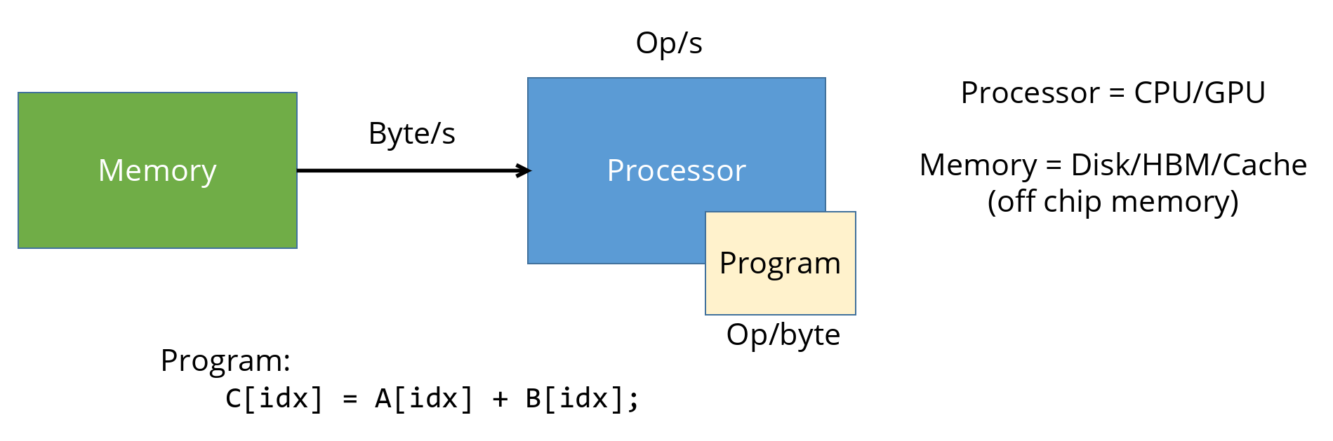
As a concrete example, consider a vector addition. For each element, we load two floating-point values from memory, add them together (the actual computation), and store the result back to memory. We will omit the store for now, since writes may not immediately consume memory bandwidth (they may first go to cache and be written back later).

In this operation, we load two floats: 4 + 4 = 8 bytes total, and perform a single arithmetic operation.

We therefore say that this program has an arithmetic intensity (AI) of:

AI = 1 op / 8 bytes = 1/8 op/byte

In other words, for every byte fetched from memory, the program performs 1/8 of an operation. This metric captures how effectively a program uses the data it moves. Arithmetic intensity is a property of the program (or its implementation/kernel).

A different performance metric describes how fast the CPU or GPU is actually executing these operations, measured in op/s. This is commonly referred to as computational performance or throughput.

Arithmetic Intensity (AI) = op/byte
How many operations are performed per byte of data moved. Also called Operational Intensity (OI).

Performance = op/s
How fast the processor is executing operations. Also called throughput (when the pipeline is full and steady) .

Note: Operations are often referred to as FLOPs (floating-point operations), since performance analysis usually focuses on floating-point workloads. For simplicity, we will use the term op throughout this article.

The Plot

We can visualize these two metrics on an X–Y plot.

• The X-axis is op/byte, which measures how well we utilize the data we fetch.
• The Y-axis is op/s, which measures how fast we are executing operations.

The Roofline plot without the roofs!

Moving to the right means we are extracting more work from each byte of data.

Moving upward means we are executing more operations per second.

In practice, many optimizations improve both metrics at once, causing the point to move diagonally up and to the right.

Improvement Strategies

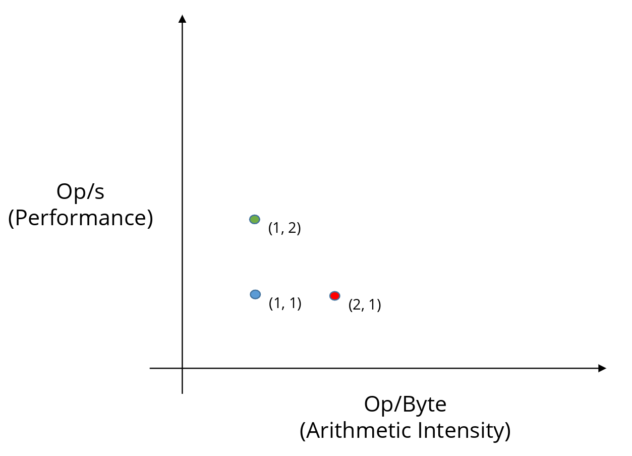
Let us first focus on a single point in this plot: the blue point at (1, 1).

This point tells us that:

• The implementation performs 1 operation per byte of data fetched (X coordinate).
• The implementation runs at 1 op/s (Y coordinate).

By itself, this does not say whether the implementation is good or bad. However, following the theme of this article - memory vs. processor limitations, there are two orthogonal ways to improve performance.

---

1. Increase arithmetic intensity (move right)

We can try to do more work per byte, i.e., increase op/byte, which moves the point horizontally to the right.

• This corresponds to moving from the blue point (1, 1) to the red point (2, 1).

How can we do more work with the same data? How about by reducing memory wastage?

A common example comes from matrix multiplication. Suppose matrix B is stored in row-major order, but the algorithm accesses it column-wise. Each load brings an entire cache line, yet only one element is used before the rest are evicted.

Accessing an element of each row means we will invalidate cache line every single time

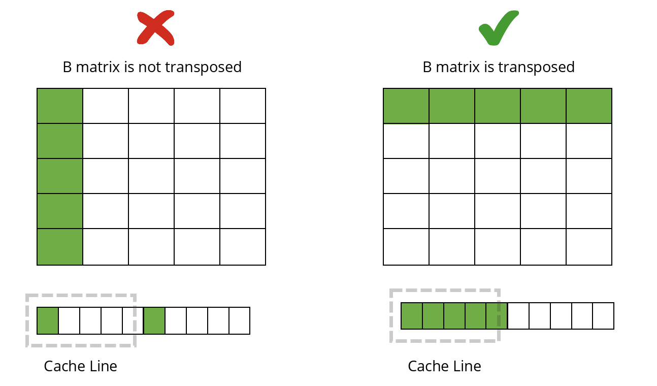
If we instead use a transposed B matrix, accesses become contiguous in memory. This improves cache reuse and allows us to perform more operations with the same bytes fetched.

As a result, arithmetic intensity increases, and the point moves to the right on the plot.

---

2. Increase computational performance (move up)

Alternatively, we can try to execute more operations per second, increasing op/s, which moves the point vertically upward.

• This corresponds to moving from the blue point (1, 1) to the green point (1, 2).

How can we increase op/s without changing the amount of data fetched?

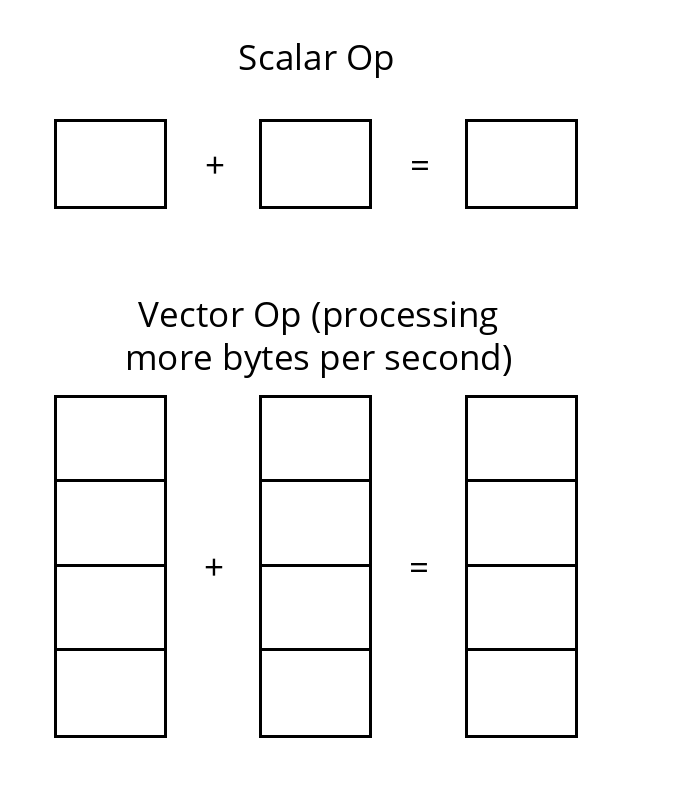
This is typically achieved through instruction-level parallelism.

• Vectorization is a classic example. Instead of performing a single scalar operation on narrow data, we operate on wider vectors, allowing multiple operations to be executed simultaneously.

Vectorizing the operation means more data is processed by a single operation

• On GPUs, another example is reducing warp divergence. If only half the threads in a warp are active, the hardware effectively wastes cycles. By restructuring the code so that all threads in a warp follow the same execution path (e.g., via warp specialization), we improve utilization of the processing units.

These techniques increase throughput (op/s) and move the point upward on the plot.

What prevents us from moving upward indefinitely along the vertical axis?

The Rooflines

Memory Roof

Let us now look at the memory bandwidth required by each point on the plot.
Bandwidth describes how fast data must move from memory to sustain a given implementation.

We can compute the required bandwidth from the slope of the line connecting the point to the origin:

\[ \text{BW} = \frac{y}{x} = \frac{\text{op/s}}{\text{op/byte}} = \text{byte/s}. \]

This is because each point represents a specific pairing of arithmetic intensity and performance. For the blue point, executing 1 op/s at an arithmetic intensity of 1 op/byte implies that the memory system must supply data at 1 byte/s, i.e., the required bandwidth is 1 byte/s.

Dividing the y value by x for each point gives us the required bandwidth we need for that implementation (point)

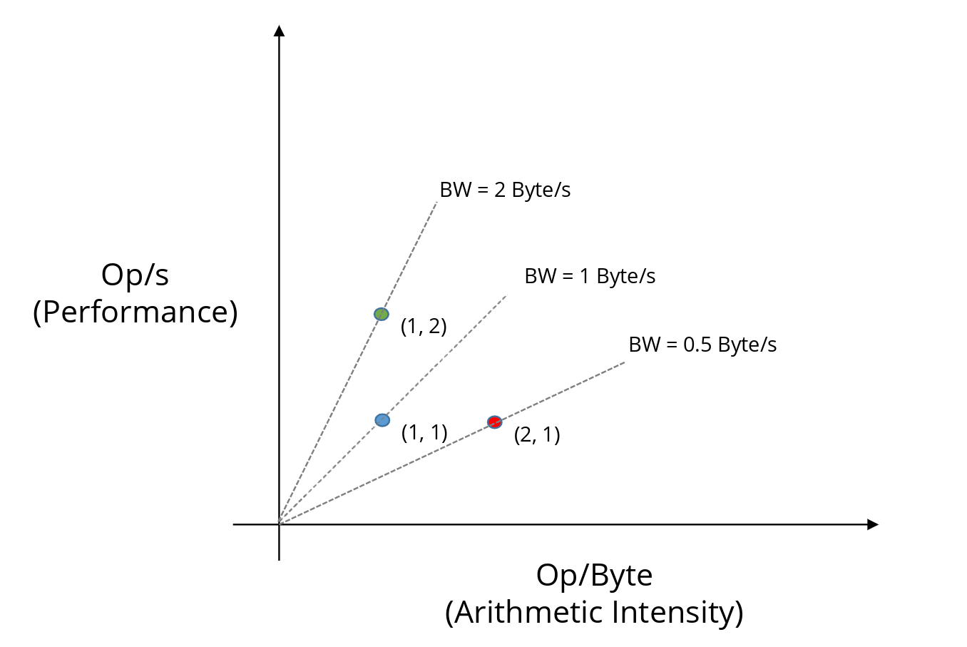
• Blue point (1, 1):
  BW = 1 / 1 = 1 byte/s

• Red point (2, 1):
  BW = 1 / 2 = 0.5 byte/s

• Green point (1, 2):
  BW = 2 / 1 = 2 byte/s

We can see that the green point requires the highest bandwidth, followed by blue, then red:

Green > Blue > Red (ordered by slope)

This means the green implementation is the most memory-intensive. In other words, to sustain that level of performance, the system must be able to deliver a very high memory bandwidth.

Now suppose the system’s peak memory bandwidth is only 1.5 byte/s. In that case, the green implementation is no longer feasible. The memory subsystem simply cannot supply data fast enough.

For an implementation, bandwidth must be lower than the system capacity

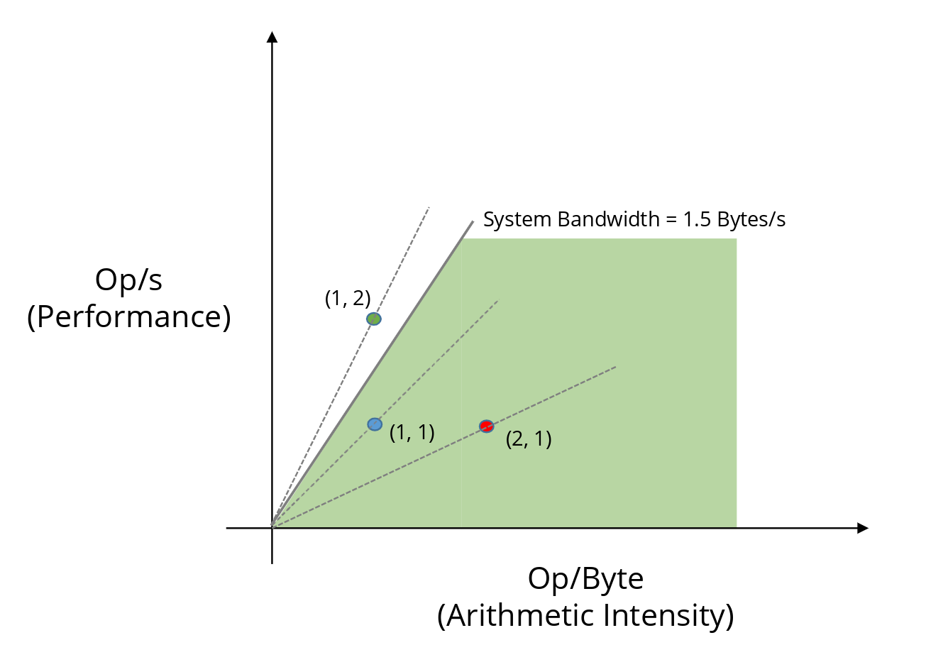
At this point, we hit a wall. Or more precisely, a roof.

This slanted line is called the memory bandwidth roof. It tells us that performance cannot increase indefinitely through techniques such as vectorization or parallelism: eventually, the implementation will be limited by how fast memory can deliver data.

---

Compute Roof

So far, this suggests that we may not be fully utilizing the data we already have. Suppose we improve arithmetic intensity (move right, toward the red point) and then try to increase performance by moving upward.

What stops us now?

For an implementation, computed performance (op/s) must also be lower than the system capacity

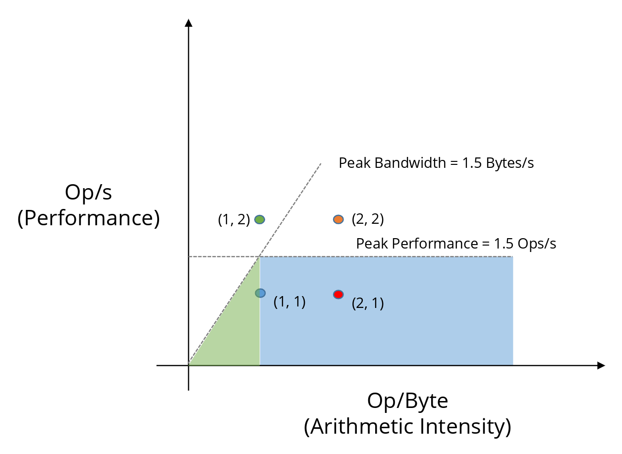
Consider an orange point at (2, 2).

• Required bandwidth = 2 / 2 = 1 byte/s, which is below the system’s peak bandwidth (1.5 byte/s).

So memory is no longer the bottleneck. However, the processor itself has a maximum rate at which it can execute operations - its peak computational performance.

If the processor’s peak performance is 1.5 op/s, then even with sufficient data, it cannot execute operations faster than that. Any point that lies on or above this horizontal limit is therefore compute-bound.

This horizontal line is called the compute roof.

---

The Roof Equation

We can summarize the entire Roofline model with a single equation:

\[ \text{Performance} = \min\left( BW_{\text{peak}} \times AI, \text{Performance}_{\text{peak}} \right) \]

This equation defines the achievable performance (y) for every possible value of arithmetic intensity (x).

• The memory-bound region corresponds to the simple line equation \(y = \text{slope} \times x\)
  \[ \text{Performance} = BW_{\text{peak}} \times AI \] where the slope is the system’s peak memory bandwidth.
• The compute-bound region is limited by
  \[ \text{Performance} = \text{Performance}_{\text{peak}} \] which already has the correct unit of op/s.

Together, these two limits form the characteristic “roofline” shape.

Summary

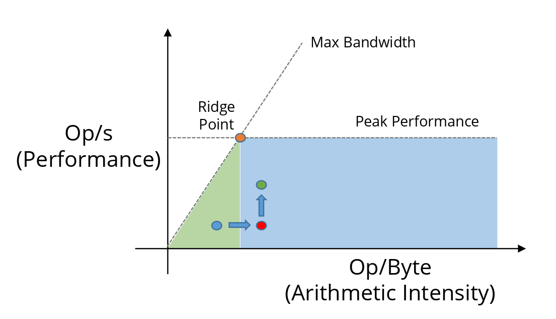
Let’s recap the whole idea and devise a solid strategy. Given an implementation (blue dot) our goal is to move it as right (higher arithmetic intensity = more FLOPs per byte transferred) and up (higher achieved FLOP/s = better utilization of the compute units) as possible.

Going Right (higher arithmetic intensity, lower bytes per OP)

These focus on reducing memory traffic relative to computation (more reuse, less movement):

1. Tiling / Blocking (cache blocking, shared memory tiling on GPU, register blocking)
2. Kernel / Operator Fusion (fewer intermediate arrays → drastically less memory traffic)
3. Better data layout (AoS → SoA, structure-of-arrays, padding for alignment, transpose tricks)
4. Exploit Cache Locality (contiguous access, temporal locality → data reuse soon after loading, spatial locality)
5. Loop fusion or fission (strategic — fuse when it increases reuse, fission when it enables better tiling/vectorization)
6. Prefetching + cache blocking together (move data into faster levels before needed)
7. In-place algorithms (avoid extra read/write of temporary buffers)
8. Algorithmic or mathematical reformulation (higher-order methods, winograd-style conv, Strassen-like matmul, etc. — trade some extra flops for far less data movement)
9. Quantization or lower precision (when acceptable — fewer bytes per value → higher effective intensity)
10. Sparsity exploitation (structured/unstructured sparsity, pruning + sparse formats → skip loading/storing zeros)
11. Data compression or lossless compression in memory (sometimes used in scientific codes)

Going up (higher OP/s, better compute utilization)

These techniques primarily improve how efficiently the processor/GPU uses its floating-point units, vector lanes, tensor cores, etc.:

1. SIMD/Vectorization (use wider vectors: AVX, AVX-512, NEON, CUDA warps with vector types)
2. Loop Unrolling (reduce loop overhead, expose more independent operations)
3. Kernel/Operator Fusion (e.g. Fused Multiply-Add → FMA, fused conv+bn+relu, elementwise + reduction chains)
4. Warp Specialization (GPU) / Thread divergence minimization
5. Prefetching (software prefetch or hardware auto-prefetch tuning — hides latency → higher issue rate)
6. Better instruction mix / throughput-bound fixes (reduce divides → use reciprocals, minimize expensive math functions)
7. Multi-threading/Occupancy (more concurrent warps/threads to hide latency and saturate functional units)
8. Use of specialized units (tensor cores, DP4A/INT8/FP16/bfloat16 paths, AMX on x86, etc.)
9. Reduce thread predication/control divergence (branchless code, mask-based ops)
10. Instruction-level parallelism (ILP) within a thread (reorder code, expose more independent ops)

Dual-impact techniques (move both right and up)

These are especially powerful because they simultaneously reduce memory pressure and improve compute efficiency:

1. Kernel Fusion / Operator fusion (very high impact on both axes)
2. Tiling + Vectorization together (typical combination in high-performance codes)
3. FMA usage (often enabled by fusion or careful coding)
4. Shared memory + warp-level tiling (GPU classic)
5. Register blocking + unrolling (CPU classic)

A good mental model is: first get the point right of the ridge point (out of the green marked memory-bound regime), then push up toward the flat compute roof. Many real optimizations alternate between these two goals as we iterate.